Scatter Plot Maker: Free Tools, Line of Best Fit and R²
A scatter plot maker is a tool that plots one dot per row of data, using two numeric columns as the x and y positions, so you can see whether the two variables are related. For most people the best free option is Google Sheets or Excel, which also add a line of best fit with its equation and R². Use Desmos for math class regressions, RapidTables for a quick plot with no account, and Datawrapper when the scatter plot goes on a web page. This guide compares those tools, shows how to read a scatter plot, and works through one example with real regression numbers.
We checked every tool in this guide on its own website or help center on November 1, 2026. The example data is fictional; the statistics were calculated from it.
When to use a scatter plot
Use a scatter plot when every item has two measurements and you want to know whether they move together: hours studied and exam score, ad spend and sales, height and weight.
| You want to show | Better chart |
|---|---|
| Whether two numeric variables are related | Scatter plot |
| How one value changes over time | Line graph |
| How categories compare | Bar graph |
| A third variable, such as company size | Bubble chart (a scatter plot where dot size is the third value) |
Google describes the use case simply: a scatter chart helps you "find out how much one variable is affected by another" (Google Docs Editors Help). For other chart types, read our graph maker guide to choosing a chart and free tool.
Free scatter plot makers compared
Checked on November 1, 2026.
| Tool | Account needed | Line of best fit | Shows equation and R² | Getting the chart out | Best for |
|---|---|---|---|---|---|
| Google Sheets | Google account | Linear, exponential, polynomial, logarithmic, power, moving average | Yes (R² needs the legend turned on) | Download as PNG, PDF or SVG | Shared data and class projects |
| Microsoft Excel | Free for Excel for the web; desktop needs Microsoft 365 | Linear, logarithmic, polynomial, power, exponential, moving average | Yes, as chart options | Copy into Office files; Save as Picture on desktop | Analysts and lab reports |
| Desmos | None | Regression templates or your own model | Shows r for linear fits, R² for others, plus residuals | Share link or image | Math and statistics classes |
| RapidTables | None | Linear, exponential or polynomial per series | Draws the line | Print or save from the browser | A quick plot with no sign-up |
| Datawrapper | Free account | Linear, quadratic, cubic, exponential, logarithmic, power or custom (Refine tab > Trend line) | Draws the line | Responsive embed; free plan exports PNG with attribution | Scatter plots on websites |
| Python (Matplotlib + NumPy) | None | Any model you code | Yes, you calculate it | Any format | Repeatable analysis |
Quick picks:
- Homework or a lab report: Google Sheets, Excel or Desmos, because you need the equation and R².
- One plot in two minutes, no account: RapidTables.
- A scatter plot for a website: Datawrapper.
- The same plot every week from new data: a short Python script.
Set up your data
Every scatter plot maker expects the same shape:
- First column: x values, the variable you think explains the other (hours studied).
- Second column: y values, the variable you think responds (exam score).
- One row per item. Each row becomes one dot.
- Numbers only. Text such as "5 hrs" breaks the plot; put units in the header.
For several groups on one plot, Google Sheets reads each extra column of y values as a new series (Google). In Excel, add each group with Select Data > Add.
Worked example: hours studied vs exam score
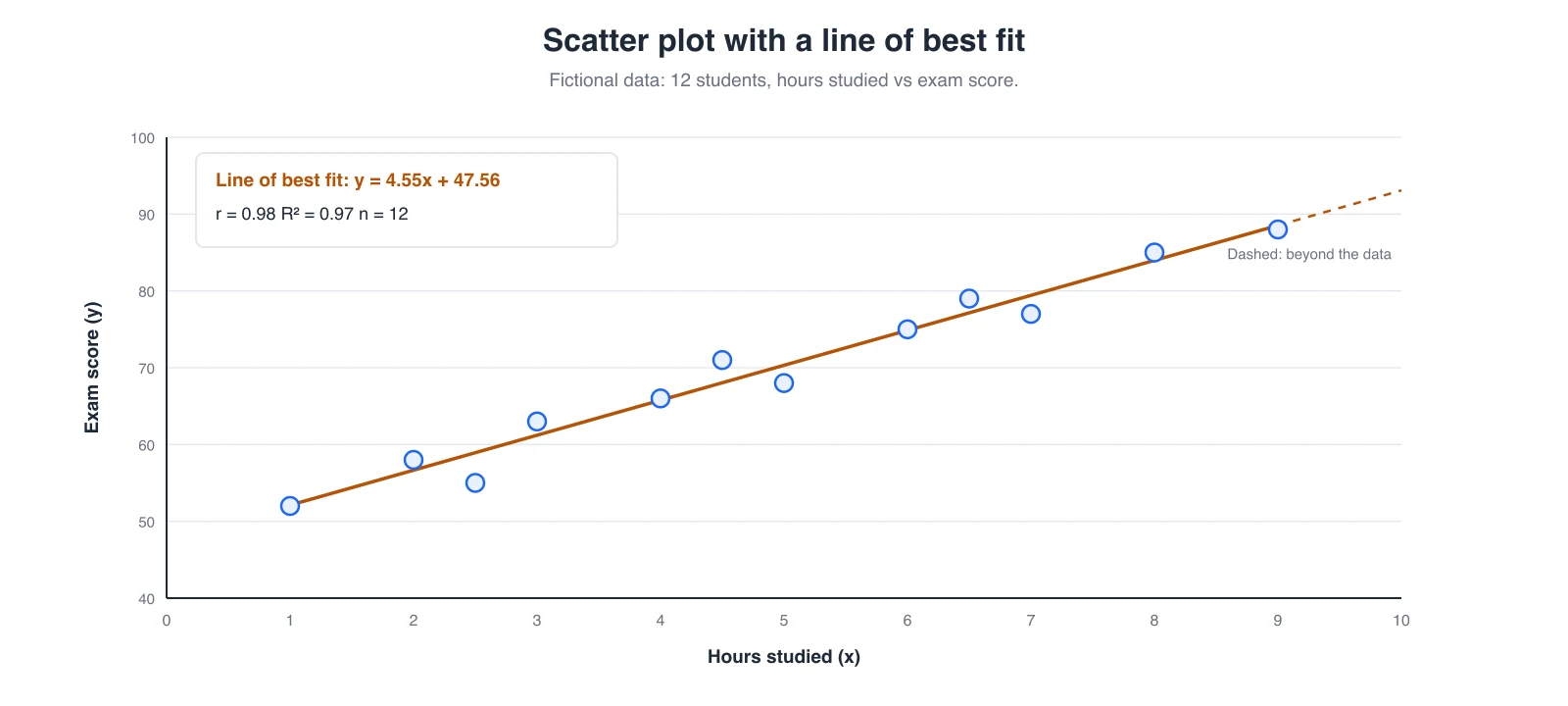
Twelve fictional students:
| Hours studied (x) | Exam score (y) |
|---|---|
| 1 | 52 |
| 2 | 58 |
| 2.5 | 55 |
| 3 | 63 |
| 4 | 66 |
| 4.5 | 71 |
| 5 | 68 |
| 6 | 75 |
| 6.5 | 79 |
| 7 | 77 |
| 8 | 85 |
| 9 | 88 |
What the numbers say:
- Line of best fit: y = 4.55x + 47.56. Each extra hour of study goes with about 4.6 more points.
- r = 0.98. A strong positive correlation. As a rough rule of thumb, values above 0.7 or below −0.7 are often called strong.
- R² = 0.97. The line accounts for about 97% of the variation in scores in this data set.
- Prediction inside the data is reasonable: at 5 hours, the line predicts about 70.
- Prediction outside the data is not: the line says 10 hours gives 93, but nobody in the data studied more than 9 hours. That is why the extension is dashed.
And what they do not say: correlation is not causation. Students who study more may also sleep better or attend more classes. A scatter plot shows that two variables move together, not why.
How to read a scatter plot
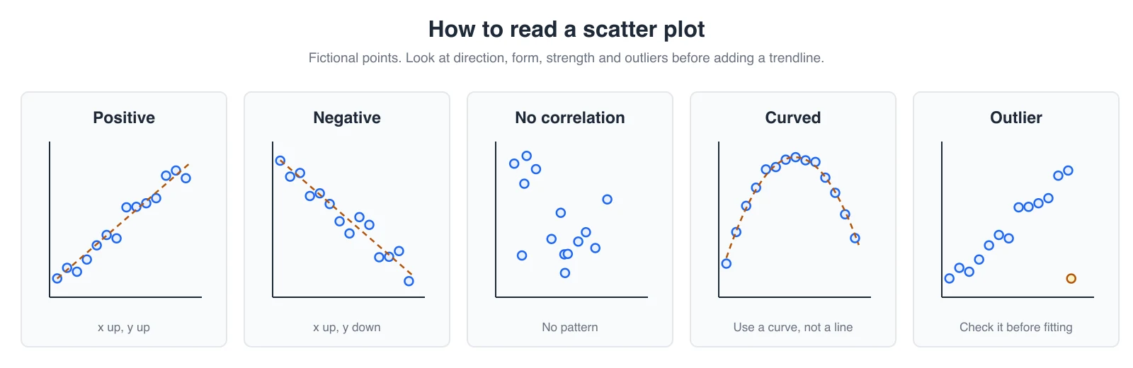
Look at four things before you add any trendline:
- Direction: do points rise (positive), fall (negative) or neither?
- Form: is the pattern straight or curved? A straight line through a curve gives a misleading fit; try a polynomial or logarithmic trendline instead.
- Strength: are points tight around the pattern or loosely spread?
- Outliers: is one point far from the rest? Check whether it is a data entry error before you remove it, and say so if you do.
Add a line of best fit in your tool
Google Sheets
- Select both columns and choose Insert > Chart, then Scatter chart on the Setup tab.
- On Customize > Series, tick Trendline and pick Linear.
- Under Label, choose Use Equation. Turn on Show R² (Sheets only shows it when the legend is on).
Excel
- Select both columns, with x values in the first column, and choose Insert > Charts > Scatter.
- Click the chart, then Chart Elements (+) > Trendline > More Options.
- In Format Trendline, tick Display Equation on chart and Display R-squared value on chart.
Desmos
- Paste the two columns into a table. Desmos names them x₁ and y₁.
- Click Add Regression, or type
y_1 ~ m x_1 + bon a new line. - Desmos shows m, b and r. Pick another model from the dropdown for curved data (Desmos Help).
TI-83 / TI-84 graphing calculator
- STAT > 1:Edit, enter x values in L1 and y values in L2.
- 2nd > Y= (STAT PLOT) > Plot1, turn it On and pick the scatter icon.
- ZOOM > 9:ZoomStat to fit the window.
- STAT > CALC > 4:LinReg(ax+b) for the line. To see r and r², turn on DiagnosticOn from the catalog (or Stat Diagnostics in the MODE menu on newer OS versions).
Python
import numpy as np
import matplotlib.pyplot as plt

x = np.array([1, 2, 2.5, 3, 4, 4.5, 5, 6, 6.5, 7, 8, 9])
y = np.array([52, 58, 55, 63, 66, 71, 68, 75, 79, 77, 85, 88])
m, b = np.polyfit(x, y, 1)
r = np.corrcoef(x, y)[0, 1]

plt.scatter(x, y)
plt.plot(x, m * x + b)
plt.title(f"y = {m:.2f}x + {b:.2f}, R² = {r**2:.2f}")
plt.xlabel("Hours studied")
plt.ylabel("Exam score")
plt.savefig("scatter.png", dpi=200)
This gives the same result as the chart above: y = 4.55x + 47.56, R² = 0.97.
Calculate the line of best fit by hand
Statistics classes often ask you to show the working. Here it is for the 12 students above, using the least-squares formulas that Sheets, Excel and Desmos use.
| Step | Formula | Result |
|---|---|---|
| Mean of x | x̄ = Σx ÷ n = 58.5 ÷ 12 | 4.875 |
| Mean of y | ȳ = Σy ÷ n = 837 ÷ 12 | 69.75 |
| Sum of cross-products | Sxy = Σ(x − x̄)(y − ȳ) | 312.125 |
| Sum of squares of x | Sxx = Σ(x − x̄)² | 68.5625 |
| Sum of squares of y | Syy = Σ(y − ȳ)² | 1,466.25 |
| Slope | m = Sxy ÷ Sxx | 4.5524 |
| Intercept | b = ȳ − m·x̄ | 47.557 |
| Correlation | r = Sxy ÷ √(Sxx · Syy) | 0.9844 |
So the line is y = 4.55x + 47.56, and R² = 0.9844² ≈ 0.97.
Check the residuals. A residual is the actual y minus the predicted y. The largest one here belongs to the student who studied 2.5 hours and scored 55: the line predicts 58.9, so the residual is −3.9. No residual is far from the rest, so there is no outlier pulling the line.
Draw a scatter plot by hand on graph paper
- Draw the x-axis and y-axis and label both, with units.
- Choose a scale that fits the smallest and largest values, with even steps (for the example: x from 0 to 10 in steps of 1, y from 40 to 100 in steps of 10). Mark the axis break if y does not start at 0.
- Plot one dot per row at (x, y). Do not join the dots.
- To sketch a line of best fit, draw a straight line with roughly equal numbers of points above and below it, passing through the mean point (x̄, ȳ), here (4.875, 69.75).
- Give the plot a title that names both variables.
Common scatter plot mistakes
| Mistake | Fix |
|---|---|
| Using a line chart for two numeric variables | Use a scatter chart, so x values are placed by value |
| Swapping x and y | Put the explanatory variable on x, the response on y |
| Forcing a straight line through a curve | Check the form first; try a polynomial or log trendline |
| Reporting a trend from a handful of points | Say how many points you have; collect more if you can |
| Extending the line far beyond the data | Show the fit only across the data range, or mark the extension |
| Thousands of overlapping dots | Use smaller, semi-transparent dots, or a heat map |
| Claiming one variable causes the other | Say "is associated with" unless you ran an experiment |
| Alt text that only says "scatter plot" | Describe the relationship, such as "scores rise about 4.6 points per study hour" |
Frequently asked questions
What is the best free scatter plot maker?
Google Sheets and Excel are the best free scatter plot makers for most people, because they also add a line of best fit with its equation and R². Desmos is best for math classes, RapidTables for a quick plot without an account, and Datawrapper for scatter plots with trend lines on websites.
How do I make a scatter plot with a line of best fit?
Put x values in the first column and y values in the second, insert a scatter chart, then add a linear trendline. In Google Sheets it is under Customize > Series > Trendline; in Excel it is under Chart Elements > Trendline. Turn on the equation and R² to show the fit.
What does R² mean on a scatter plot?
R² (the coefficient of determination) shows how much of the variation in y the trendline accounts for, from 0 to 1. An R² of 0.97 means the line accounts for about 97% of the variation in that data set. It does not prove that x causes y.
What is the difference between r and R²?
r, the correlation coefficient, runs from −1 to 1 and shows the direction and strength of a straight-line relationship. For a simple linear fit, R² is r squared, so it is always between 0 and 1 and has no sign.
What is the difference between a scatter plot and a line graph?
A scatter plot places every point by two numeric values to show a relationship. A line graph spaces x values evenly and connects points to show change over time or another ordered sequence.
Can a scatter plot show more than two variables?
Yes. Color the dots by group to add a category, or use a bubble chart, where dot size shows a third number. Google Sheets and Excel both make bubble charts.
How do you find the line of best fit by hand?
Calculate the means of x and y, then the slope m = Σ(x − x̄)(y − ȳ) ÷ Σ(x − x̄)² and the intercept b = ȳ − m·x̄. The worked table above shows each step for 12 data points.
Is a scatter plot the same as a scatter graph or XY graph?
Yes. Scatter plot, scatter graph, scatter chart, scatter diagram and XY graph all mean the same chart.
Keep your analysis in one place
A scatter plot is usually one step in an analysis: the data, the chart, the fit and your conclusion belong together. In AFFiNE you can keep the source table, the exported chart and your notes in one doc, or lay out several plots side by side on the AFFiNE whiteboard.
Update note (November 1, 2026): This article was first published in June 2025 and rewritten in November 2026. We replaced a long, generic overview with a dated comparison of six scatter plot makers checked on each vendor's site, an original worked example with regression results we calculated (y = 4.55x + 47.56, R² = 0.97), a guide to reading scatter plots, steps for adding a line of best fit in Google Sheets, Excel, Desmos, a TI-84 and Python, a by-hand calculation with residuals, graph-paper steps, and new FAQs on r and R². We replaced the shared cover and unlabeled images with original graphics. AI tools assisted with drafting, and the content was reviewed and edited by the AFFiNE team.